
Estimate two-photon excitation from pulsed-laser settings or solve for the average power needed to reach a target excitation chance per pulse.
Advanced options
How to use our Two-Photon Absorption Calculator
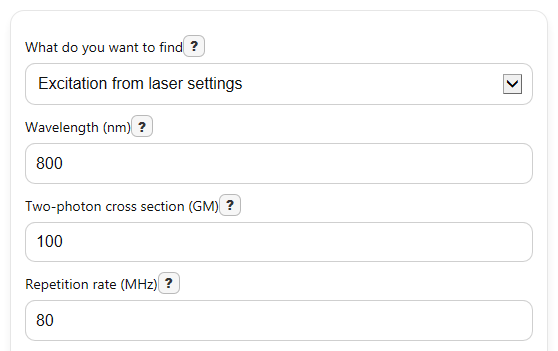
- Choose "What do you want to find" and enter the shared laser inputs: "Wavelength (nm)", "Two-photon cross section (GM)", "Repetition rate (MHz)", "Pulse width (fs)", and "Beam waist radius (um)".
- If you picked excitation mode, fill in "Average power (mW)". If you picked power-needed mode, fill in "Target excitation chance per pulse (0 to 1)" instead.
- Open "Advanced options" only if you need them, then set "Pulse shape", "Beam profile factor", or how to show very big or very small numbers.
- Click "Calculate" and read the main result first, then check "Peak intensity at focus", "Peak photon flux", and any "Note" to see whether your setup may be outside the simple weak-excitation range.
- Sanity-check the output by asking whether the beam size is a radius, not a diameter, and whether doubling "Beam waist radius (um)" or "Average power (mW)" changes the result in the direction you expect.
Definitions
Two-photon cross section (GM): A standard measure of how strongly a molecule responds to two-photon excitation. Larger GM usually means easier excitation under the same laser conditions.
Repetition rate (MHz): How many laser pulses happen each second. For example, 80 MHz means 80 million pulses per second.
Pulse width (fs): The duration of one pulse in femtoseconds. Shorter pulses usually give higher peak power for the same average power.
Beam waist radius (um): The focused beam radius, not diameter. Because area depends on radius squared, this input strongly affects intensity.
Average power (mW): The time-averaged laser power across many pulses.
Pulse energy (nJ): The energy in one pulse, found from average power divided by repetition rate.
Peak intensity at focus (W/cm^2): Estimated highest power per area at the focus. Two-photon effects rise strongly as this value increases.
Peak photon flux: The number of photons passing through each square centimeter each second at the pulse peak.
Excitation chance per pulse: The estimated probability that one pulse excites one molecule in this simple model.
Common mistakes and quick fixes
Mistake: Entering beam diameter into "Beam waist radius (um)".
Fix: Enter the radius at focus. If you only know diameter, divide it by 2 before using "Beam waist radius (um)".
Mistake: Typing 10 for "Target excitation chance per pulse (0 to 1)" when you mean 10%.
Fix: Enter probabilities as decimals between 0 and 1, so 10% should be entered as 0.1.
Mistake: Using "Average power (mW)" while the calculator is set to solve for power.
Fix: In power-needed mode, the main input is "Target excitation chance per pulse (0 to 1)", and "Average power needed" is the output.
Mistake: Forgetting that "Two-photon cross section (GM)" must be greater than 0.
Fix: Enter the published value in GM for your fluorophore and wavelength, and make sure the number is positive.
Mistake: Mixing up laser timing units in "Repetition rate (MHz)" or "Pulse width (fs)".
Fix: Enter repetition rate in MHz and pulse width in femtoseconds exactly as labeled, not in Hz, kHz, ps, or ns.
Mistake: Ignoring a very high "Excitation chance per pulse" or the "Note" output.
Fix: Treat high probabilities as a sign that the simple estimate may be less reliable, and use the warning note to decide whether to lower power or re-check inputs.
Limitations & Key Assumptions / Boundary Conditions
- This calculator uses a simple pulsed-laser estimate based on average power, repetition rate, pulse width, beam waist radius, and two-photon cross section.
- The model assumes the entered "Beam waist radius (um)" is the focused radius. Using diameter instead causes a 4x area error.
- Results are most reliable in the weak-excitation range. When "Excitation chance per pulse" gets high, saturation and other non-ideal effects can make the simple estimate less accurate.
- The "Pulse shape" and "Beam profile factor" settings are correction-style inputs, not a full optical system model.
- The calculator does not include losses from objectives, windows, alignment, dispersion, scattering, or sample-specific local-field effects.
- The output depends strongly on the published "Two-photon cross section (GM)", which can vary with wavelength, environment, and measurement method.
- Very small beam waists or extreme target probabilities can produce mathematically valid but physically unrealistic power or intensity estimates.
Methodology
Core method
This calculator first converts the entered laser settings into per-pulse quantities, then uses a standard two-photon rate estimate based on photon flux squared. The main idea is simple: the same average power can behave very differently when repetition rate, pulse width, or beam waist changes.
E_pulse = P_avg / f_rep
P_peak = E_pulse / τ
I_peak = spatial factor x P_peak / (π x w0^2)
F_peak = I_peak / (h x c / λ)
k_2 = σ2 x F_peak^2
P_exc = 1 - exp(-k_2 x τeff)
R_exc = P_exc x f_rep
Here, τ is pulse width in seconds, w0 is beam waist radius in centimeters, λ is wavelength in meters, h is Planck's constant, c is the speed of light, and σ2 is the two-photon cross section after converting GM to cm^4 s photon^-1 molecule^-1. The calculator uses 1 GM = 1e-50 cm^4 s photon^-1 molecule^-1.
Power-needed mode
When you choose the backward solve, the calculator rearranges the same model to find the average power needed for your target per-pulse probability.
P_avg = (f_rep x τ x area x (h x c / λ) / spatial factor) x sqrt((-ln(1 - P_target)) / (σ2 x τeff))
This keeps the forward and backward modes consistent. If the target probability is extremely close to 1, the required power rises very fast because the logarithm term grows without bound.
Mini-example
Using 800 nm, 100 GM, 80 MHz, 100 fs, 0.5 um beam waist radius, and 10 mW average power gives a pulse energy of about 0.125 nJ and a peak power of about 1250 W. With the default ideal beam factor, that leads to a peak intensity near 1.59e11 W/cm^2 and an excitation chance per pulse of about 0.00449. Multiplying by 80 million pulses per second gives about 3.59e5 excitation events per second.
Assumptions behind the estimate
The simple probability expression works best when excitation per pulse is well below 1 and the setup stays in a weak-to-moderate excitation regime. At higher probabilities, real samples can differ because of saturation, bleaching, pulse broadening, imperfect focusing, transmission losses, and wavelength-dependent cross-section data [1].