
Enter your HPLC gradient and sequence plan to calculate mobile phase A and B preparation amounts, pumped volume, runtime, and solvent cost.
Advanced options
Calculation details
Table of contents
How to use our HPLC Mobile Phase Blend and Run Cost Calculator
- Copy every cumulative time and percent B point from the instrument method into the Gradient program, including holds, wash steps, return to the starting blend, and re-equilibration.
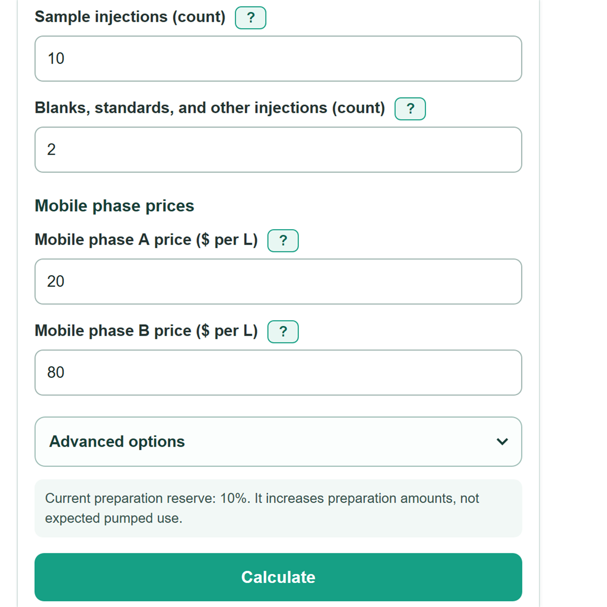
- Enter the constant Flow rate (mL/min), then enter Sample injections and Blanks, standards, and other injections from the planned worklist.
- Enter Mobile phase A price ($ per L) and Mobile phase B price ($ per L) using your lab's prepared-phase cost or current purchase records.
- Open Advanced options to change Preparation reserve (percent) or add Solvent-waste disposal price ($ per L) if your lab uses a volume-based disposal charge.
- Click Calculate, then check that Injections included in the plan matches the worklist and that Expected mobile phase pumped by the sequence is lower than Total mobile phase to prepare when a reserve is used.
Definitions
Gradient program: A list of cumulative time points and percent B values that describes the mobile-phase composition over one complete programmed run.
Percent B: The share of mobile phase B in the pumped blend at a time point. Mobile phase A is calculated as 100 minus percent B.
Flow rate (mL/min): The constant volume pumped each minute. One mL/min for 10 minutes pumps 10 mL total.
Preparation reserve (percent): Extra volume added to the A and B preparation targets above expected sequence use. It is not treated as pumped solvent.
Expected mobile phase pumped by the sequence: The calculated A plus B volume for all planned injections before reserve.
Solvent-waste disposal price ($ per L): An optional volume-based disposal charge applied to expected pumped volume, not to unused reserve.
Common mistakes and quick fixes
Mistake: Leaving the wash, return, or re-equilibration period out of the Gradient program.
Fix: Add every programmed stage through the final cumulative time so Expected mobile phase pumped by the sequence covers the full cycle.
Mistake: Entering percent A in a Gradient program row that asks for percent B.
Fix: Enter percent B only; the calculator finds A as the remaining percentage.
Mistake: Counting only Sample injections and forgetting blanks or standards.
Fix: Put blanks, standards, controls, and planned repeats in Blanks, standards, and other injections.
Mistake: Treating Total mobile phase to prepare as the exact amount the instrument will pump.
Fix: Use Expected mobile phase pumped by the sequence for method-derived use; Total mobile phase to prepare also includes Preparation reserve (percent).
Mistake: Using the same number for Mobile phase A price ($ per L) and Mobile phase B price ($ per L) without checking the actual prepared-phase costs.
Fix: Price A and B separately so Planned sequence solvent and waste cost reflects the blend composition.
Mistake: Entering a price such as 1,01 for Mobile phase A price ($ per L).
Fix: Use commas only for thousands separators and a decimal point for cents, such as 1.01 or 1,001.01.
Limitations & Key Assumptions / Boundary Conditions
- The calculation assumes one constant Flow rate (mL/min) for the entire Gradient program. It does not model methods with flow changes by segment.
- It treats composition changes between adjacent Gradient program rows as linear. Enter a row at each hold, step, wash, return, and re-equilibration change.
- It uses the programmed gradient timing as entered. It does not adjust for dwell volume, gradient delay, mixing behavior, or when a gradient reaches the column.
- Programmed sequence runtime excludes autosampler delays, injection setup, data processing, instrument startup, and unentered work.
- Preparation reserve (percent) is a planning choice for items such as priming, transfer loss, or small sequence changes. It does not predict actual unused solvent.
- Planned sequence solvent and waste cost includes only entered A and B prices and an optional volume-based disposal price. It excludes columns, labor, maintenance, instrument cost, and overhead.
Methodology
Gradient volume calculation
Each pair of adjacent Gradient program rows is one time segment. The calculator uses the average percent B at the two ends of that segment, so a straight composition change is treated as a linear change.
segment_B_minutes = (end_time_min - start_time_min) * (start_percent_B + end_percent_B) / 200
integrated_B_minutes = sum of all segment_B_minutes
program_duration_min = final gradient time
integrated_A_minutes = program_duration_min - integrated_B_minutes
The integrated A and B minutes are then multiplied by the constant flow rate to find mL used in one injection.
A_per_injection_mL = flow_rate_mL_per_min * integrated_A_minutes
B_per_injection_mL = flow_rate_mL_per_min * integrated_B_minutes
Sequence and preparation calculation
All sample and other injections use the same entered program. Their counts are added before the per-injection volumes and runtime are scaled.
total_injections = sample_injections + other_injections
sequence_A_mL = A_per_injection_mL * total_injections
sequence_B_mL = B_per_injection_mL * total_injections
total_sequence_use_mL = sequence_A_mL + sequence_B_mL
total_prepare_mL = total_sequence_use_mL * (1 + preparation_reserve_percent / 100)
The same reserve multiplier is applied to A and B separately. For example, a 0 to 10 minute segment changing from 5% B to 95% B averages 50% B. At 1 mL/min, that segment uses 5 mL B and 5 mL A per injection. For 12 injections, it uses 60 mL of each before reserve. A 10% reserve changes each preparation target to 66 mL.
Cost calculation
Prices are entered in dollars per liter, while solvent use is in mL, so the calculation divides mL by 1,000. The optional disposal rate is applied only to expected pumped volume.
sequence_cost = sequence_A_mL * A_price_per_L / 1000 + sequence_B_mL * B_price_per_L / 1000 + total_sequence_use_mL * waste_price_per_L / 1000
cost_per_injection = sequence_cost / total_injections
When total injections is zero, sequence use, preparation volume, runtime, and costs are zero. Cost per injection is shown as $0 to avoid dividing by zero.
What the math includes
The method uses only entered gradient rows, a constant flow rate, planned injection counts, prices, and optional reserve or disposal values. It does not add unentered priming, dwell-volume corrections, flow-program changes, delays, or fixed laboratory costs.